Memory Proportional Progressive Precision: A New Approach to the LLM Inference Memory Wall

How to serve more LLM and agent requests on the same hardware without sacrificing quality.

This article presents a new method for serving large language model and agentic inference. The problem it addresses is well known to anyone operating large language models or AI agents at scale and it is an expensive one. The binding constraint on modern inference is not compute but memory. Every request accumulates a working state as it executes and that state rather than the arithmetic is what saturates the accelerator and limits how many requests can be served concurrently. The prevailing response has been to procure more of the scarcest and most expensive memory available. This method proposes an alternative.

This article is a deliberate pivot from my recent writing. My prior articles worked largely at the level of models and how they learn. The Builder’s Guide for Agentic AI Design laid out patterns for composing agentic systems that actually ship. Confidence Aware Reinforcement Learning examined how a large language model can carry a sense of its own predictive confidence through uncertain and dynamic environments. Reinforcement Learning for Feature Compatibility Optimization proposed an adaptive learning framework using distributed parameter sharing and automated feedback. Each of those addressed how a model reasons or how it is trained. This article goes a different direction. Not at the model but at the economics of running it once it is trained. The best architecture and the best training still meet a hard physical ceiling at serving time and that ceiling is memory. It is worth stepping away from learning algorithms to examine the constraint that increasingly governs what any of these systems can actually do in production.

My approach is termed Memory Proportional Progressive Precision (MPP). It represents a new treatment of the inference memory wall. Rather than provisioning every request for the worst case MPP allocates memory in proportion to the difficulty of each individual request and does so under an explicit quality guarantee rather than through unbounded approximation. The result is a substantial reduction in memory per request and a multiplicative gain in throughput on existing hardware. The method is straightforward to state generally across model architectures and can be integrated into an existing serving stack. The sections that follow set out the problem, the mechanisms, and the mathematics underlying MPP’s behavior and a path to a working prototype.

The LLM Memory Wall

Modern inference runs on GPUs and comparable accelerators. Each device pairs its compute cores with a small pool of high bandwidth memory (HBM) adjacent to the die and a larger pool of conventional DRAM on the host. For a request to execute at full speed its working state must reside in HBM. Spilling to host DRAM incurs a significant bandwidth and latency penalty. HBM capacity per device is limited, grows slowly across hardware generations and costs substantially more per gigabyte than conventional DRAM, which is itself under sustained price pressure. HBM is therefore typically the first resource to be exhausted and additional capacity cannot simply be purchased since each device accommodates only a fixed amount. This condition is commonly referred to as the memory wall.

The severity of the constraint follows from the origin of the working state. It grows over the course of a request and the form of that growth depends on the model.

Transformers and LLMs. The key value attention cache grows with every token generated and for long contexts becomes the single largest object in memory.

Diffusion and iterative generators. Latents and intermediate feature maps are held across every denoising or sampling step.

Ranking and recommendation. Candidate sets feature vectors and partial scores expand as the query broadens.

Speech and voice. Beam hypotheses and acoustic or language model context grow with utterance length.

Agents and tool users. Retrieved context tool outputs and accumulated scratch state grow as the agent works through a task and each sub call can add more.

The Source of the Waste

The critical observation is that most requests do not require the full working state to produce a correct result. For a document assistant a query such as “how many sections does this contract have” is answerable from a small portion of the input whereas “reconcile every payment clause against the appendix schedule” may require the entire document in context. A coding agent asked to rename a variable needs almost no context. The same agent asked to trace a defect across a repository needs a lot more. Request difficulty varies by orders of magnitude across a realistic workload.

Conventional serving treats every request as though it were the hardest case. It materializes full precision state unconditionally and therefore incurs the worst case memory cost even for answers that a fraction of that state would have produced exactly. Reducing quality to recover the cost is not a viable remedy because an answer returned quickly but incorrectly is generally worse than no answer at all. The system consequently over provisions on every request.

Conventional serving sizes every request for the worst case. MPP sizes each request for what it actually requires and certifies that the answer meets the quality target before releasing it.

Allocating Memory in Proportion to Difficulty

MPP serves an LLM or agent request by first materializing its working state at the lowest precision tier sufficient to meet a quality bound declared by the caller. It escalates to a higher precision tier at greater memory cost only when a quality estimate indicates escalation is necessary and only as far as necessary. Memory is thus allocated according to the difficulty of the individual request rather than the worst case. This yields lower expected memory per request and on a fixed budget and a multiplicative increase in throughput together with a guarantee that every released answer falls within the declared bound.

The contribution is not the notion of producing an approximate result and then refining it. That approach is well established. It is the enclosure of that notion within a memory budgeted control loop that wraps the model governed by a declared quality bound and a sound quality estimator. Precision escalates as a joint function of a memory governor and a bound on the output error, and the request terminates at the first tier that clears the bound. Quality is embedded in the memory saving mechanism itself rather than applied as a separate downstream check.

Figure 1: the MPP control loop. A request arrives carrying a declared quality bound ε. The precision controller functioning as a memory governor selects a tier. The state materializer allocates working state for it. the engine executes. The quality estimator returns a certified bound. If the bound falls within ε the result is released otherwise the controller advances to the next tier allocates additional state and repeats.

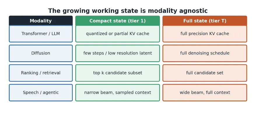
MPP is independent of any particular architecture. It requires only two properties and both hold across essentially all of machine learning. First the working state can be materialized at several precision tiers whose memory cost increases with the tier. Second output quality does not decrease as the tier increases. Figure 2 aligns the compact tier and the full tier against four model types.

Figure 2: the same compact versus full state split across four model types. MPP handles all of them through one precision tier abstraction.

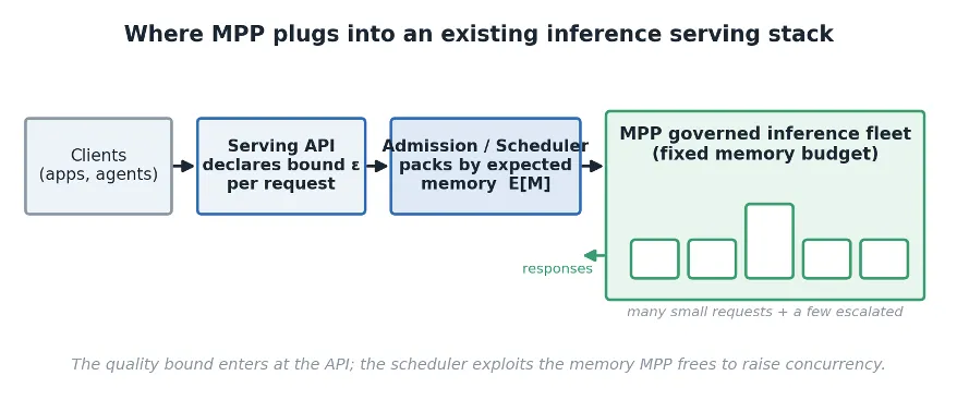
The method also integrates into a conventional serving deployment with minimal modification. The only externally visible change is that a request may carry a declared quality bound through the serving API. The controller and estimator wrap the existing model and execution engine and the scheduler is adapted to pack requests by their expected memory rather than their worst case footprint. Figure 3 indicates where the components sit.

Figure 3: where MPP slots into an existing inference serving stack. The quality bound enters at the API and the scheduler puts the memory MPP frees toward running more requests at once on the same fleet.

The Mechanism

A formal statement makes the memory saving and the quality guarantee precise. Consider a single request whose answer can be produced at any of T ordered precision tiers from t = 1 (most compact) to t = T (full precision). A tier is an abstraction over whatever parameter controls state size in a given system. In a large language model or agent it is the fraction of context retained, the number of bits in a quantized cache, the size of a scored candidate set, the width of a search beam or the number of iterative steps.

Materializing state through tier t consumes M(t) of memory comprising a fixed base footprint (the model weights and base context) plus the increment contributed by each tier along the way. Because no increment is negative M(t) increases monotonically with t and a higher tier never costs less memory than a lower one. This monotonicity is what makes early stopping a genuine saving rather than a gamble.

Memory accumulates as state is added. M₀ is the base footprint and each tier’s increment is non negative so M(t) rises with t.

Let the result at tier t be denoted ŷ(t) and let y* be the exact full precision answer. The error q(t) measures the distance of the tier t answer from exact. The second assumption is that additional state never degrades the result so q(t) decreases monotonically or at worst holds constant as t increases and the full tier attains the tightest tolerance the system can achieve. Additional context precision or search can only sharpen the result.

Error does not increase as precision rises and the full tier T reaches the minimum error the system can achieve.

Early stopping is made safe by the estimator and specifically by its reporting a certified upper bound on the true error rather than an optimistic estimate. Before a compact answer is trusted the system must hold proof that the error cannot exceed a computed value. That value q̂(t) must be at least as large as the true and unknown error q(t). In practice the estimator may be a confidence interval derived from a sampled subset, a quantization error bound, a rank stability margin for a top k query, or for an LLM a bound on the shift in the output token distribution. The estimator must never understate the error. This is what converts a heuristic judgment into a defensible guarantee.

The estimator’s reported bound is never below the true error. This soundness property is what elevates the method from an approximation to a guarantee.

The controller releases the answer at the first and therefore lowest memory tier whose certified bound falls under the caller’s tolerance ε. This stopping tier t* is the smallest t at which the bound is within ε. If no tier below the full tier clears ε the rule escalates to T which clears the tightest bound by construction. The system allocates exactly as much memory as the quality target demands and no more.

t* is the cheapest tier that is provably good enough. Escalation halts the instant the certified bound drops under ε.

Figure 4: escalation halts at the cheapest tier that satisfies the bound. Green bars denote memory M(t), the descending line is the certified bound and the dashed line is the declared bound ε. This request stops at tier 3 so tiers 4 and 5 are never materialized.

Because most requests terminate well below the full tier, expected memory per request is a probability weighted average over stopping tiers dominated by the low cost tiers where the majority of traffic resolves. It falls well below the worst case M(T) that conventional serving incurs on every request. The magnitude of the saving is determined entirely by the traffic distribution. The greater the share of requests that stop early the lower the expected memory.

Expected per request memory is a probability weighted sum over stopping tiers well below the full tier cost when most requests stop early.

Because the estimator is sound and the rule releases only when the bound falls within ε the answer honors the declared quality bound with high probability. The residual failure probability δ reflects the slack in the estimator and is zero for a perfectly sound estimator. This property distinguishes MPP from ordinary best effort approximation.

The released result honors the declared bound with probability at least 1 minus δ where δ reflects the estimator’s soundness.

Expected Impact

The two benefits are directly coupled. Every gigabyte not spent on a low difficulty request is a gigabyte available to serve another request concurrently. On a fixed memory budget the number of requests that fit simultaneously is governed by expected per request memory. Reducing that quantity raises concurrency and throughput together, which is what lets a large language model or agent fleet serve more sessions per accelerator.

Concurrency C is the memory budget divided by expected per request memory. Throughput scales with C over expected latency. Reducing expected memory raises both.

Figure 5 quantifies this on a representative workload. When the compact state occupies approximately 38 percent of the full footprint and only a minority of requests escalate to full precision, per request memory falls by more than 60 percent and throughput on identical hardware increases by a factor of 1.6 to 2.6 depending on the escalation rate. Figure 6 presents the same effect as memory packing. Where a worst case fleet accommodates three full size requests MPP accommodates numerous compact requests alongside the escalated request within the same budget.

Figure 5: left, peak working state memory per request under worst case provisioning against MPP. Right, throughput on a fixed memory budget as the share of requests that escalate to full precision changes. Memory saved on easy requests turns directly into concurrency.

Figure 6: the same memory budget serving far more requests. Conventional serving reserves each request’s worst case footprint. MPP packs in many compact requests and a few escalated ones for the same memory.

Application Across AI

The control loop is identical in every case. Only the state parameter and the estimator change. This uniformity is what makes MPP a general pattern rather than a workload specific optimization.

Long context LLM serving: For a summarization or question answering request tier 1 attends over a key value cache that has been quantized or partially evicted and the estimator bounds the perturbation that quantization or eviction could introduce into the output distribution. When the bound falls within ε the response is produced from the compact cache. When the request is sensitive to the omitted precision the system escalates to a fuller cache. Because the key value cache is the largest memory consumer in transformer serving sizing it per request against the quality target accounts for the majority of the saving.

Agentic workflows: An agent addressing a broad task accumulates retrieved documents tool outputs and intermediate reasoning and this context is the primary source of growth. Tier 1 executes the task over a tightly pruned context and the estimator assesses whether the conclusion is stable with respect to the omitted material for example by determining whether additional context would alter the tool calls the agent selected. Routine tasks resolve on the pruned context. Only those whose outcome depends on the omitted material escalate to a fuller context and its associated memory. The same construction applies to sub agent delegation. A parent assigns a child a scoped task at tier 1 and re-executes it with richer context only if the child’s result is not certified stable.

Retrieval augmented question answering: Tier 1 answers from the highest ranked retrieved chunks and the estimator provides a margin on whether lower ranked chunks could alter the answer. When the top chunks clearly contain the answer the full retrieved set is never loaded into context, when they do not the system escalates.

Recommendation and ranking: A recommender returns a user’s top items from a candidate pool numbering in the hundreds of thousands. Tier 1 scores a coarse aggressively pruned set within a small footprint and the estimator is a rank stability margin assessing whether any pruned candidate could plausibly displace one that made the cut. For most users the head of the ranking is unambiguous and the answer is produced from the pruned set. Only the closely contested cases escalate to a larger pool.

Speech and voice: A transcriber executes a beam search whose memory grows with beam width and language model context. Tier 1 uses a narrow beam and the estimator is the score gap between the leading hypothesis and the runner up. Routine commands resolve on the narrow beam, ambiguous or noisy audio in which competing hypotheses are closely scored escalates to a wider beam for that utterance alone.

Relationship to Existing Techniques

MPP shares surface features with several established techniques and the distinctions are instructive. Cache eviction and offloading reduce memory but do not condition on a declared quality bound and offer no per request quality guarantee.

Approximate query processing and early exit or anytime inference trade accuracy for speed, generally lacks a certified caller controlled error bound and are not organized as a memory budgeted escalation over precision tiers.

Adaptive quantization varies precision but is not governed by a per request quality target with a certified stopping rule. MPP is the combination of these elements. It brings together ordered precision tiers, a sound estimator, a declared bound stopping rule and a scheduler that converts the freed memory into concurrency. The individual components exist in prior work. Unifying them under a single quality contract is what makes the method effective.

A Path to a Prototype

A full implementation is not required to evaluate the approach. A practical first implementation proceeds as follows. Select a workload in which request difficulty varies materially. Long context LLM question answering or an agentic task loop is a strong candidate. Begin with two tiers compact and full rather than an extended ladder. Select a single estimator that can be certified sound for that workload even a conservative one since a loose but sound bound still saves memory on low difficulty requests. Expose a single quality parameter on the API with a sensible default so that callers who do not set it still receive correct answers. Measure the stopping distribution on production traffic before introducing additional tiers. In practice the majority of the benefit is realized with two tiers and one estimator. The extended ladder is a refinement rather than a prerequisite.

Conclusion

Memory and specifically the scarce and costly HBM on which accelerators depend is now the binding constraint on large language model and agentic inference, and conventional serving wastes it by sizing every request for the worst case. MPP eliminates that waste by allocating memory in proportion to the precision each request requires under a declared quality bound with a sound estimator gating every release. Expected memory per request falls throughput on identical hardware and rises by a multiple. Quality is held within a bound rather than traded for speed. The method is architecture agnostic and integrates into existing serving stacks. It is also straightforward to prototype with two tiers and a single estimator. For any organization or product operating large language models or agents at scale where memory is the ceiling, MPP warrants serious consideration.